
 I came up with this content back in 2024, and made a school math project regarding this topic. However, I enjoyed making the project so I believe it would also serve as a nice, short blog post. Pre-requisites are understanding polar coordinates, basic calculus, trigonometry, and a bunch of algebra. Despite my best attempts at explaining how some of the more elementary ideas in this post contribute to the proofs, it is best if you are familiar with them.
Enjoy the math ramblings of a high-schooler!
I came up with this content back in 2024, and made a school math project regarding this topic. However, I enjoyed making the project so I believe it would also serve as a nice, short blog post. Pre-requisites are understanding polar coordinates, basic calculus, trigonometry, and a bunch of algebra. Despite my best attempts at explaining how some of the more elementary ideas in this post contribute to the proofs, it is best if you are familiar with them.
Enjoy the math ramblings of a high-schooler!
Logarithmic spirals are a class of mathematical shapes described by a simple mathematical equation. Despite the elegance & simplicity of how they are generated, they have some extremely interesting properties and characteristics which warrants a small case study on them. This blog post will look at some of those characteristics which most piqued my interest and present an attempt to prove their.
Namely, we will look at how logarithmic spirals are congruent under rotation and scaling, and hence self-similar, and the fact that their pitch angles are constant.
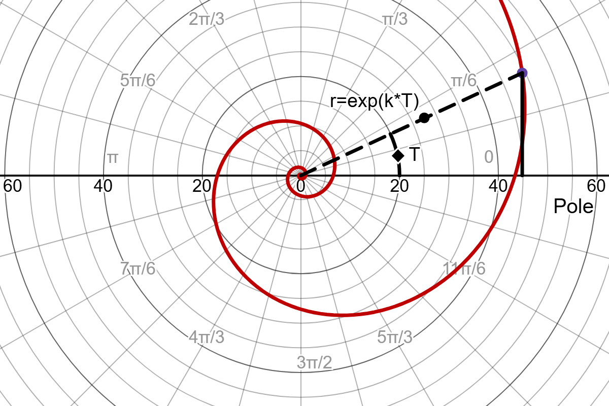
We begin by defining how a logarithmic1 spiral is constructed:
Analyzing this equation qualitatively, we see that this means that as $\theta\to\infty$, the radius or distance from the origin, $r\to\infty$ too. But it does get hard to imagine exactly what this curve looks like, so let’s try plotting this on Desmos. Click on me!
Now that we can visualize what this curve looks like, we notice a few different things. First off, if you tried manipulating $k$, you would’ve noticed that increasing its magnitude increases the amount by which the spiral “opens” up. When $k$ is near 0, the curve collapses near the origin and looks more and more like a circle.
This should motivate you to notice that $k$ doesn’t just determine how fast the spiral grows, but also how much it opens up with each turn.
And as it turns out, there is indeed a beautiful link between the constant $k$ and the “openness” of the curve— a concept mathematicians call the pitch angle of the spiral.
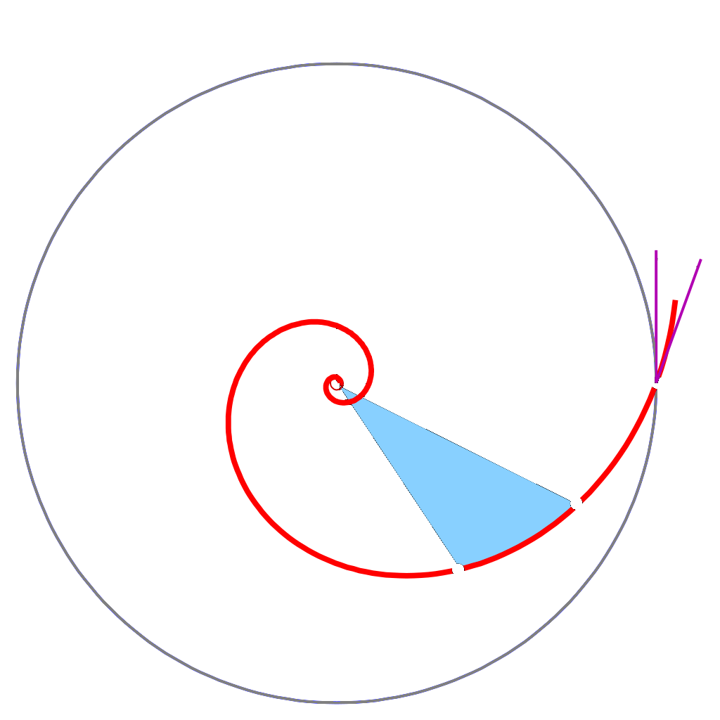
More rigorously, we can state that the pitch angle is the angle between the tangent to the circle at point $P$ and the tangent to the spiral at that same point.
Back at our Desmos graph, open up the first folder and follow the instructons. Now, manipulate $\theta_0$ and observe the two tangents drawn to the spiral and circle. Does the angle, $\alpha$, change as you move along the spiral? Does it change for changing $k$?2
As it turns out, the relationship between $k$ and $\alpha$ is quite elegant:
This result is quite significant because it intuitively tells us that the “openness” of the curve depends only on the choice of $k$, and nothing else. And this $\alpha$ does not change for any spiral— it’s constant!
Property One: Constant Pitch Angles
Proof. We begin by observing that the pitch angle may also be redefined in terms of tangent lines to each of the spiral and circle — that is, the angle between their tangents at some point in the polar plane $(r, \theta)$. Denote each of these lines $L_s$ and $L_c$ for the spiral and circle respectively. Notice these lines can be written as (in cartesian coordinates): 3
For slopes $m$ on points $(x_s , y_s), (x_c, y_c)$ on the spiral and circle. All that is essential is finding the slopes. We know, however, that:
Since they are tangent to the same point, the spiral and circle’s intersection. And also by the product rule of differentiation. 4
Where the derivatives are representations of how fast the $x$ and $y$ coordinates change with respect to changes in $\theta$, respectively.
And from the chain rule 5 , it follows that:
For any and all polar equations and curves.
For the spiral, we have $r = e^{k\theta}$, so $r’ = ke^{k\theta}$: 6
For the circle, $r = r_c$, where $r_c$ is a constant radius of our liking. Hence, the derivative $r’ = 0$:
Now, recall we defined the pitch angle $\alpha$ as the angle between the tangents to the spiral and circle. Luckily, this angle depends only on the slopes of those tangents, which we have found in $(1)$ and $(2)$. The formula is as given:
At this point, we take an important step which I think younger me described well:
Now substitute back \(a\) and \(b\):
Using \(\cot(x)\sin(x) = \cos(x)\):
So finally, $\alpha = \arctan(k)$, which was to be demonstrated!
And yet again, our result makes sense, remember our Desmos graph showed that the angle between the spiral and circle tangents remained constant everywhere.
Property Two: Rotations are the same as Scaling
Open up the second folder (pt. 2), and follow the instructions listed. Slide $d$; what happens to the curve? Notice that it is being rotated, but what is intriguing is that this also looks exactly the same as zooming in or out on the curve. Try it out!
Another important property of these spirals is that rotating a spiral has the same effect as scaling (zooming in or out) it. Namely:
Proof. Consider $r(\theta-d)$.
Which was to be demonstrated, in our case $a=e^{-kd}$
Which also proves something called self-similarity.
Property Three: Self-similarity
Self-similarity occurs when a scaled shape is congruent to its original shape by rotation. That is, zooming in or out on it is the same as rotating the curve by some angle.
Luckily, we have just proven exactly that, so all logarithmic sprials are, by extension, self-similar!
For example, consider a logarithmic spiral $r(\theta)=e^{\theta/2}$ rotated $90^\circ=\frac \pi 2$. We can show, because of the previous property:
Hence, rotating it 90 degrees had the same effect as zooming out by 0.456 units.
And you can do this in the opposite direction— any scaling can be converted into a rotation.
Golden Spirals and $\varphi$: Special Logarithmic Spirals!
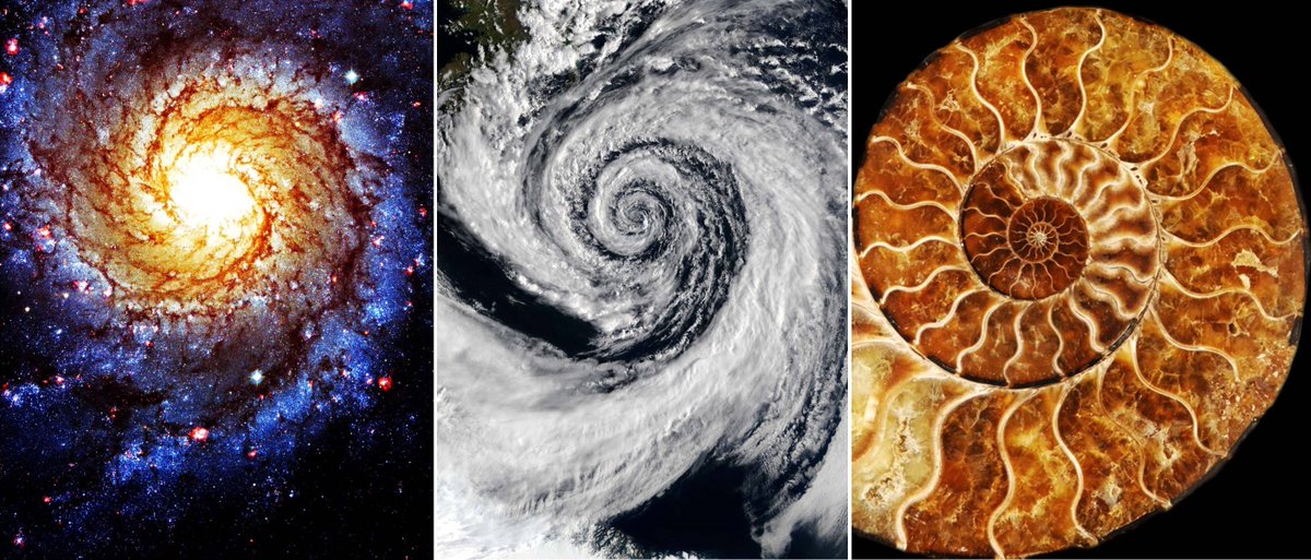
You’ve probably seen those viral posts on social media—gushing over the “divine” beauty of nature and the supposed presence of the golden ratio everywhere. Cue a zoomed-in image of a sunflower or a nautilus shell, complete with an overlaid golden spiral and a caption like “See? Math is the language of the universe!” I find these posts pretty pretentious: they do nothing to attempt explaining the math, and attribute any spiral looking shape to the golden spiral, which is just wrong.
The golden spiral, depicted on the left, is indeed a type of logarithmic spiral with a unique $k$, however often times in nature, spirals are not golden! That is, their $k$ is not the same as the “golden” $k$.
These posts have glamorized the golden ratio without giving any credit to the way these shapes are even generated— through logarithmic spirals. The rest of this blog will be dedicated to finding a polar form of the golden spiral— in the logarithmic spiral form we defined previously.
Mathematically, we can denote this as The Golden Spiral being $r(\theta)=e^{k\theta}$ such that:
And we need to find $k$:
This is great! Now we know $k\approx 0.306$, which means that the golden spiral has: 7
And plugging this back into $r(\theta)$:
And that brings it to an end! In the very last folder (pt. 3) on Desmos, you should see the Golden Spiral’s equation. Go ahead and plot it!
Hopefully this blog post has inspired a newfound love in you for logarithmic spirals— the true actors behind all of those “Nature is Magnificent!” posts you see on social media. And more importantly, I hope you learnt something new.
-
This definition may not provide much insight into why these spirals are named as such, but with a bit or rearranging, we see that logarithms are indeed involved in these spirals; namely when we solve for $\theta$:
$$r=e^{k\theta}\implies \ln(r)=k\theta\implies \theta=\frac{\ln(r)}{k}$$Regardless, I believe calling these spirals exponential or growth spirals is more suiting than the unintuitive logarithmic spiral, but I digress. ↩
-
The answers to those questions are no, and yes, respectively. ↩
-
I suspect another way to do this would be to convert the lines into polar form, this way the use of chain rule is eliminated and we could do some analysis on the direct derivatives instead. Left as an exercise to you! ↩
-
$$\dv{x}\qty[f(x)g(x)]=f'(x)g(x)+f(x)g'(x)$$
-
$$\dv{x}\qty[f(g(x))=f'(g(x))g'(x)]$$
-
$$\dv{x}\qty[e^x]=e^x$$
-
which, if you pull out your protractor and ruler and measure on most of those viral nature posts, should be approximately true. ↩